A Brief Summary on Neural Style Transfer

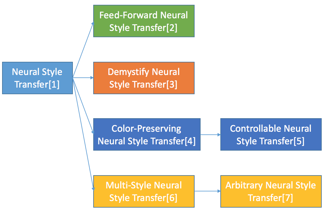
Neural Style Transfer is a fascinating yet mysterious area in computer vision. The opening paper by Leon A. Gatys et al. was published at 2015. Since then, numerous progress has been made in this area, bringing more and more fascinating features as well as enlightenment about how and why it works. In this blog post, I would like to summary several papers on this topic to draw a brief sketch about the developments in recent years as shown in Figure 1.

Opening Paper

The opening paper A Neural Algorithm of Artistic Style and Image Style Transfer Using Convolutional Neural Networks were out at 2015. Thanks to the dramatic development on CNNs (Convolutional Neural Networks), Leon A. Gatys et al. were able to separately capture image content and style using pre-trained CNN for object recognition and transfer style from one image to the other.

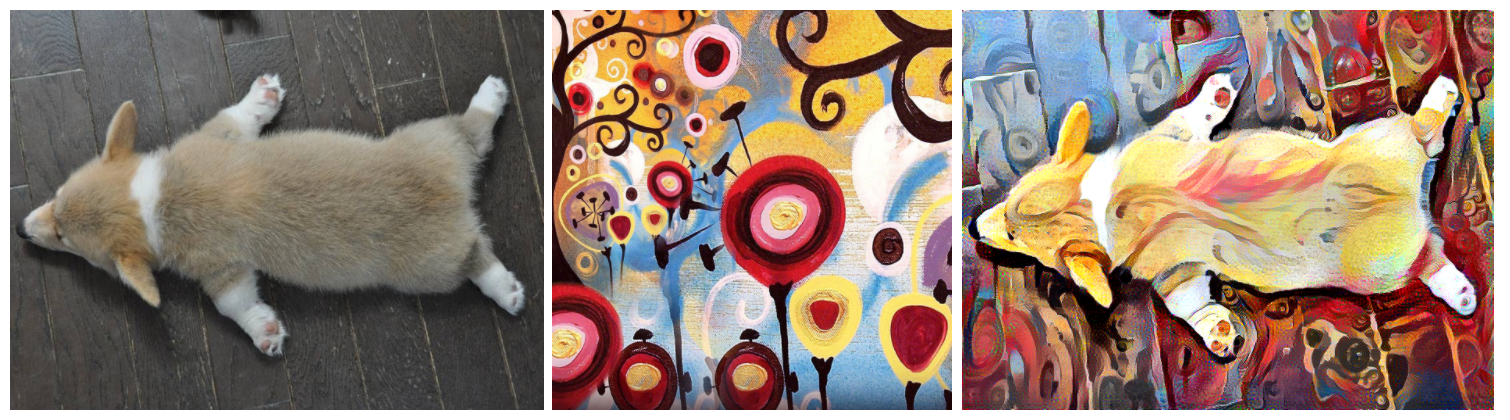
Task. In neural style transfer, one provides two images, a content image (left in Figure 2) and a style image (middle in Figure 2). Then the style transfer algorithm combines the style of the style image and content of the content image to generate a new image(right in Figure 2). This requires the separately capture of image content and style.

Capturing Image Content. CNNs are known as brilliant feature extractors. It captures low-level pixel information in shallow layers as well as high-level semantic information in deep layers. So to capture the image content information, it’s sufficient to use the feature maps by CNNs to represent image content. Thus we define the content loss as the mean square distance between the feature maps:

In which \(\vec{p}\) and \(\vec{x}\) are the original image and the generated image. \(F\) and \(P\) are their feature maps from the pre-trained VGG net in layer \(l\).

Capturing Image Style. Image style is a ill-posed definition. It’s even hard to give a specific definition verbally. An intuition is that the style of a painting(or a painter) should be irrelevant to content as well as location, so one might use a statistics over the whole feature map to represent the style of an image. This introduces the Gram Matrix which is defined as:

Given a \(C \times H \times W\) feature map. Its corresponding Gram Matrix is a \(C \times C\) matrix, with \(C_{ij}\) computed as the element-wise product and summation across feature map in channel \(i\) and channel \(j\). So it can be interpreted as the correlation between feature map \(F_i\) and \(F_j\).

We define the style loss as a weighted sum of the mean square errors between the Gram Matrices computed in layer \(l_1, l_2, ..., l_n\).

Training. The first Neural Style Transfer Algorithm is characterized as an optimization problem. Starting with a noise image, one feeds this image to the pre-train VGG net and calculate the style loss and content loss between this image and the style and content image respectively, then backpropagates the gradient all the way back to this noise image to push it closer to our target image. Repeating this optimization process many iterations, we shall get an image combining the content and style from the content image and style image. An example result is shown in Figure 2.

Drawbacks. This opening paper shows the a fantastic application of CNNs. Yet it tackles this problem by an optimization process, so it’s inefficient and can’t be applied in real world such as a phone APP. Also, why Gram Matrix can capture style of an image is kind of a myth to be revealed.

Feed-Forward Style Transfer

One issue about neural style transfer is that it needs many optimization iterations to generate a transferred image. Johnson et al. tackled this problem by training a network to complete the style transfer task. Their network architecture is shown in Figure 3. Using the same style and content loss as the opening paper, their transformer network receives a content image \(x\) and generates a target image \(\hat{y}\), \(\hat{y}\) as well as the style image \(y_s\) and content image \(y_c\) are then fed into the pre-trained VGG net to compute the style and content losses. Gradients from these two losses are back-propagated into the generated image and then used to train the transformer network. When testing, one only needs to feed the content image into the transformer network to get a transferred image. Thus the transfer task can be completed within one feed forward other than many feed-forward and backward iterations.

Demystify Neural Style Transfer

Why does Gram Matrix work? Li et al. proved that minimizing the style loss based on Gram Matrix is equivalent to minimizing the Maximum Mean Discrepancy with the second order polynomial kernel. Thus the essence of neural style transfer is to match the feature distributions between the style images and the generated images. Other than the Maximum Mean Discrepancy with the second order polynomial kernel, the optimization can also achieved by other kernels such as the linear kernel and Gaussian kernel.

Additionally, they also proposed a style loss by aligning the BN statistics (mean and standard deviation) of two feature maps between the style images and the generated images.

where \(\mu_{F^l}^i\) and \(\sigma_{F^l}^i\) are the mean and standard deviation of the \(i^{th}\) feature channel among all the positions of the feature map in the layer l for the generated image, while \(\mu_{S^l}^i\) and \(\sigma_{S^l}^i\) correspond to the style image. Image generated by minimizing the BN statistics based loss is shown in Figure 4. It has comparable performance with the Gram Matrix based loss.

Multi-style Transfer

Although fast neural style transfer accelerate the speed of Neural Style Transfer, one has to train a transformer network for each style. Dumoulin et al. observed that the parameters \(\gamma\) and \(\beta\) in the Instance Normalization layer can shift and scale an activation \(z\) specific to painting style \(s\). Conventional Instance Normalization can be represented as :

where \(x\) is the feature map of the input content image from layer l, \(\mu\) and \(\sigma\) are \(x\)’s mean and standard deviation taken across spatial axes. \(\gamma\) and \(\beta\) are learned parameters to shift and scale this feature map.

While in the proposed method which was called Conditional Instance Normalization, \(\gamma\) and \(\beta\) are expanded to \(N \times C\) matrix, with \(N\) represents the number of styles and \(C\) represents the channel number. To normalize \(x\) to a specific style \(s\), one just normalize \(x\) as:

where \({\gamma}_s\) and \({\beta}_s\) is the \(s^{th}\) row of \(\gamma\) and \(beta\), specializing to represent style \(s\). The process can be figured below:

This paper confirms the observation from Demystify Neural Style Transfer that the the Instance Normalization (A specific process of Batch Normalization when batch size equals to 1) statistics can indeed represent a style.

Another interesting paper is by Chen et al.. They trained a feed-forward style transfer network on multiple styles by using Styles Bank. A style bank is a composition of multiple convolutional filters, with each corresponds explicitly to a style. To transfer an image into a specific style, the corresponding filter bank is operated on top of the intermediate feature embedding produced by a single auto-encoder. Their network architecture is shown in Figure 6:

An image \(I\) is fed into the auto-encoder \(\varepsilon\) to get feature map \(F\). \(F\) is then convolved with each filter bank \(K_i\) to get new feature maps \(\tilde{F_i}\) specific to style \(i\). Those feature maps are then fed into the decoder \(D\) to get all transferred images. To train the auto-encoder as well as styles bank, two losses are utilized. One is the perceptual loss same as Feed-Forward Style Transfer, the other is the MSE loss of image reconstruction. This significantly reduce parameters needed for each style, from a whole transformer network to just a convolution filter. Also it supports incremental style addition by fixing the auto-encoder and training new filter specific to the new style from scratch.

Arbitrary Style Transfer

A farther step towards Multi-style transfer is arbitrary style transfer. Although conditional instance normalization can enable a transformer network to learn multiple styles, the transformer network’s capability has to increase as the number of styles it captures. A super goal of style transfer is that given a content image as well as a style image, one can get the transferred image within a single feed-forward process without a pre-trained transformer network on this style. Xun et al. proposed Adaptive Instance Normalization to achieve this. What we know from Multi-style Transfer is that the \(\gamma\) and \(\beta\) in the Instance Normalization layer can shift and scale an activation \(z\) specific to painting style \(s\). So why not just shift and scale the content image’s feature map to align with the style image in the training process ? This Adaptive Instance Normalization does exactly this:

where \(x\) is the feature map of the input content image. \(\mu(x)\), \(\mu(y)\) and \(\sigma(x)\), \(\sigma(y)\) are the mean and standard deviation of \(x\) and style image \(y\).

Their network architecture is slightly different from the feed-forward style transfer and multi-style-transfer transfer. The encoder is composed of few layers of a fixed VGG-19 network. An AdaIN layer is used to perform style transfer in the feature space. A decoder is learned to invert the AdaIN output to the image spaces.

Controllable Style Transfer

The last line of style transfer I would like to go through is style transfer that preserving color or other controllable factors such as brush stroke. I will mainly talk about color preserving, details about other controllable factors can be found in Preserving color in neural artistic style transfer. Color preserving style transfer means to preserve the color in content image while transfer the texture style from the style image to the content image. There are two approaches proposed by Gatys et al.. The first one is that for the style image \(S\) , first use color histogram matching algorithm to generate a new style image \(S'\) which matches the color histogram of the content image. Then use \(S'\) as the style image and perform conventional neural style transfer algorithm with content image \(C\). The other approach is to perform style transfer only in the luminance channel, then concatenate generated luminance channel with I and Q channel from the content image. Results are shown in Figure 8. From my own experience, the luminance-only style transfer performs better than the histogram matching algorithm since the latter one relies on how histogram matching algorithm works.

References

1. Gatys L A, Ecker A S, Bethge M. A neural algorithm of artistic style[J]. arXiv preprint arXiv:1508.06576, 2015.
2. Johnson J, Alahi A, Fei-Fei L. Perceptual losses for real-time style transfer and super-resolution[J]. arXiv preprint arXiv:1603.08155, 2016.
3. Li, Yanghao, et al. “Demystifying Neural Style Transfer.” arXiv preprint arXiv:1701.01036 (2017).
4. Gatys, Leon A., et al. “Preserving color in neural artistic style transfer.” arXiv preprint arXiv:1606.05897 (2016).
5. Gatys, Leon A., et al. “Controlling Perceptual Factors in Neural Style Transfer.” arXiv preprint arXiv:1611.07865 (2016).
6. Dumoulin, Vincent, Jonathon Shlens, and Manjunath Kudlur. “A learned representation for artistic style.” (2017).
7. Huang, Xun, and Serge Belongie. “Arbitrary Style Transfer in Real-time with Adaptive Instance Normalization.” arXiv preprint arXiv:1703.06868 (2017).
8. Chen, Dongdong, et al. “Stylebank: An explicit representation for neural image style transfer.” arXiv preprint arXiv:1703.09210 (2017).